Analysis of exchange rate volatility in Bolivia

Executive summary

This analysis was developed in Python using a two-state Hidden Markov Model (HMM), estimated from 524 observations of daily returns. The results allow for the identification of latent volatility regimes in the USDT/BOB parallel market, revealing a fragile equilibrium in which risks materialize mainly through infrequent episodes of high volatility. These episodes have the potential to accelerate the depreciation of the Bolivian boliviano, especially in contexts of heightened macroeconomic uncertainty.

Main results

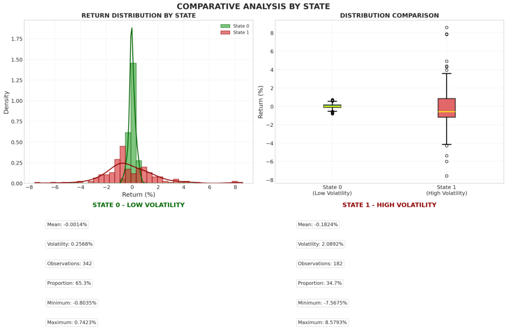
Identified regimes: The model distinguishes two volatility regimes. State 0, the low-volatility regime, accounts for 65.3% of the observations and is characterized by average returns of −0.0014% and low volatility of 0.2568%, prevailing during periods of stability. In contrast, State 1, the high-volatility regime, represents 34.7% of the cases, with average returns of −0.1824% and significantly higher volatility of 2.0892%—approximately eight times greater—associated with stress episodes featuring extreme movements of up to ±8.5%.
Market dynamics: Both regimes exhibit high persistence, with probabilities of remaining in the same state of 90.6% for low volatility and 83.3% for high volatility. The average duration is approximately 11 days in the stable regime and 6 days in the unstable regime. In the long run, the market remains 64.1% of the time in the low-volatility regime and 35.9% in the high-volatility regime.
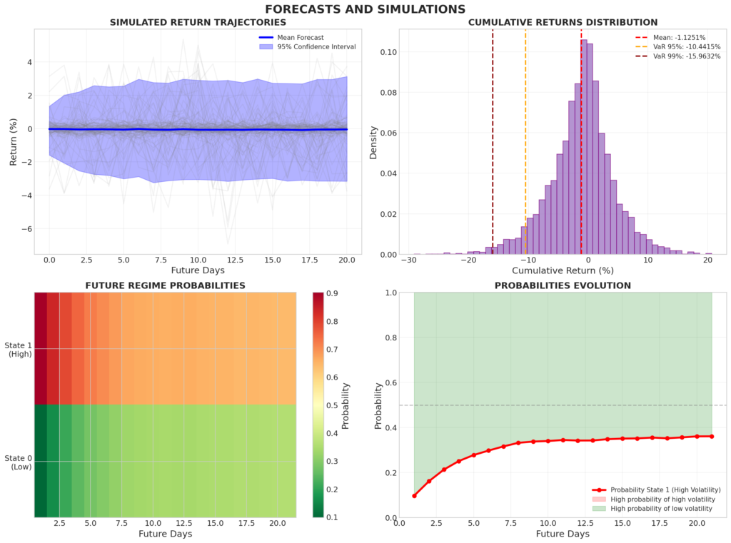
Risk assessment: Starting from the current low-volatility regime, 21-day simulations anticipate slightly negative cumulative returns, with a mean of −1.25%. However, there are significant tail risks: the 95% Value at Risk (VaR) is −10.44%, and the 99% VaR is −15.96%. Likewise, the probability of transitioning to a high-volatility regime gradually increases to around 35%, indicating greater vulnerability to adverse shocks.

About the data

The database integrates bid and ask prices from both the official and parallel markets, using the digital dollar USDT as a proxy for the parallel exchange rate. The data have daily frequency and cover the period from August 2, 2024, to January 7, 2026, with a total of 524 observations. The central variable of the analysis is the selling price of the boliviano against the dollar in the parallel market.

Exploratory Data Analysis

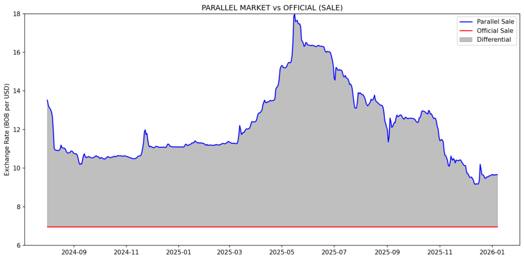
During the second half of 2024, the parallel exchange rate moderated from levels close to 13.5 BOB/USDT to around 10.5 BOB/USDT, remaining relatively stable in early 2025. Starting in March 2025, a sharp episode of depreciation of the Bolivian boliviano was recorded, reaching a peak close to 18 BOB/USDT in May, followed by a gradual correction between June and December 2025. The period closed within an approximate range of 9.5 to 10 BOB/USDT. This behavior reflects a scenario of exchange rate stress associated with deteriorating expectations, constraints on the supply of foreign currency, and increased precautionary demand for dollars. Nevertheless, despite the subsequent partial relief, the parallel exchange rate remains well above the official rate, confirming the structural nature of the exchange rate gap and the persistence of distortions in the foreign exchange market.

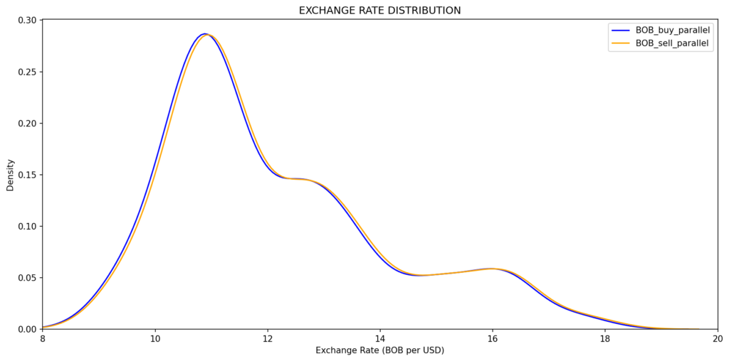
The analysis of the distribution of the exchange rate in the parallel market confirms the existence of distinct pricing regimes. The presence of a multimodal distribution, with concentrations around 10–11, 12–13, and 15–16 BOB/USDT, reflects the alternation between periods of relative stability and episodes of high tension. Moreover, the similarity between bid and ask prices suggests that fluctuations are driven mainly by macroeconomic factors and expectations, rather than by operational frictions in the market.

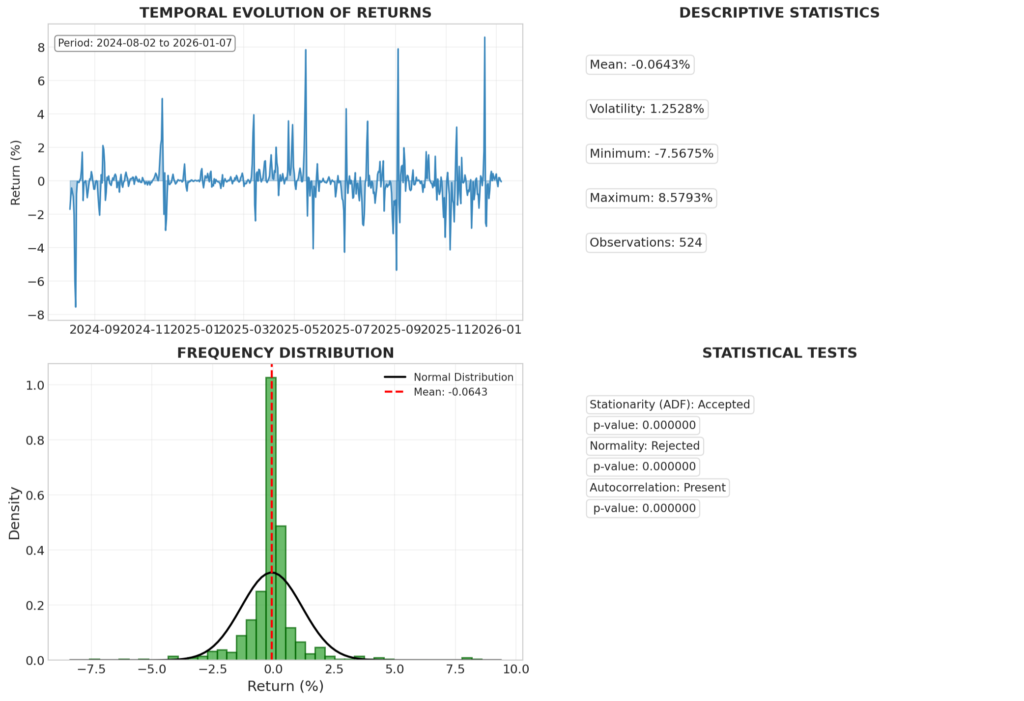
For proper analysis, the variable retorno_paralelo was constructed to represent the daily return of the parallel exchange rate in percentage terms, calculated as the daily logarithmic variation of the selling price. Its time evolution exhibits several volatility spikes, with a negative mean of −0.0643%, volatility of 1.2528%, a minimum of −7.5675%, and a maximum of 8.5793%. The distribution concentrates most returns around zero, with heavy tails.

Statistical tests confirm that the parallel exchange rate return series is stationary (ADF −10.8556, p = 0.0000), non-normal (D’Agostino K² = 189.226, p = 0.0000), and exhibits significant autocorrelation (Ljung–Box = 82.708, p = 0.0000). These results indicate leptokurtosis, asymmetry, and temporal dependence, thereby validating the use of the HMM model to capture hidden dynamics and volatility patterns in the market.

Hidden Markov Model

A two-component (regime) HMM with full covariance and 200 iterations is estimated, yielding the following results, which show no significant variation across different initializations:

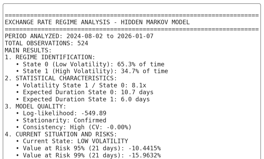
Log-likelihood: −549.8906
Random seeds: 42, 123, 456, 789, 999
Log-likelihood standard deviation: 0.000797

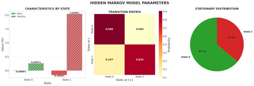
Accordingly, the bar chart displaying state-specific means and volatilities indicates that State 0 exhibits a mean return of −0.0088% and volatility of 0.2601%, while State 1 records a mean return of −1.1604% and volatility of 2.036%. The transition matrix reveals high persistence, with a 0.906 probability of remaining in State 0 and 0.833 in State 1, alongside low cross-transition probabilities of 0.094 and 0.167. The stationary distribution indicates that the market spends 64.1% of the time in State 0 and 35.9% in State 1.

These results reflect a predominant low-volatility regime with near-zero returns, contrasting with a high-volatility regime characterized by significant losses, and show that both regimes are persistent and long-lasting over time.

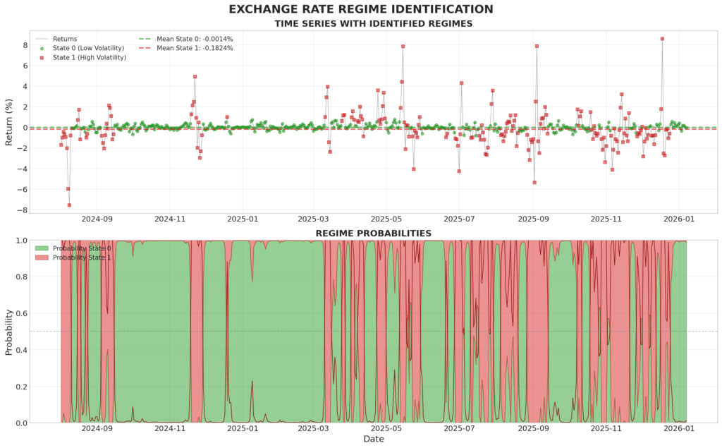
The time series of exchange rate regimes shows that State 0 (low volatility) comprises 342 observations, equivalent to 65.3%, while State 1 (high volatility) includes 182 observations, representing 34.7%. Returns shown in green correspond to periods of low volatility, whereas returns in red indicate high volatility, with mean values represented by dashed lines. Transition probabilities alternate between regimes, displaying abrupt shifts during volatile periods, particularly in 2025. Thus, the market exhibits stable periods interspersed with episodes of instability that capture significant downturns, reflecting the underlying dynamics of volatility regimes.

The following charts display overlapping distributions, where State 1 (high volatility) is clearly more dispersed, and the boxplots highlight the presence of outliers associated with this regime. The metrics confirm higher risk in State 1, while State 0 is interpreted as a stable regime with returns close to zero. Specifically, the results are as follows: for State 0 (low volatility), the mean is −0.0014%, volatility is 0.2568%, with 342 observations (65.3%), a minimum of −0.8035% and a maximum of 0.7423%; for State 1 (high volatility), the mean is −0.1824%, volatility is 2.0892%, with 182 observations (34.7%), a minimum of −7.5675% and a maximum of 8.5793%, resulting in a volatility ratio of 8.1 times.

20-Day Simulation Results: the average daily return is −0.0243% on the first day and −0.0470% at the end of the period. The 21-day Value at Risk (VaR) stands at −10.44% at the 95% level and −15.96% at the 99% level, reflecting extreme risks. The simulated return paths are shown in gray with a narrow confidence band, with the cumulative distribution centered at −1.2515%. The VaR thresholds are clearly marked, and the initial probabilities favor the low-volatility regime, although they decline slightly over time, while the overall evolution indicates persistence in low volatility.

Summary of Results

Conclusions

The two-state Gaussian Hidden Markov Model (HMM) is consolidated as a robust tool for analyzing the dynamics of the USDT/BOB exchange rate in the parallel market, showing a stable fit with a log-likelihood of −549.89 and high reproducibility across multiple initializations. Its ability to capture non-normality, heavy tails, and autocorrelation positions it as a superior approach relative to linear models, allowing for precise identification of latent volatility regimes in highly unstable environments such as Bolivia.

In the Bolivian context of January 2026, characterized by a persistent gap between the official exchange rate of 6.96 BOB/USD and the parallel rate close to 9.60 BOB/USDT, the results reflect a fragile economic equilibrium. While the predominance of the low-volatility regime suggests transitory stability, the economy remains exposed to external shocks and internal factors that could amplify depreciation episodes, with spillover effects on inflation and financial stability.

In this context, the use of regime-switching models such as the HMM is key to anticipating transitions, assessing stress probabilities, and designing proactive hedging strategies, positioning it as a strategic instrument for both policymakers and private agents in Bolivia.